7.1 Introduction

 

The heart of the present theory is that the light has a medium of propagation. Thus, Maxwell would have written his famous equations in a Preferred Frame of Reference that I call Maxwell’s Referential or also Light Referential because the light is propagating really, physically at the same constant speed c and this in all the directions in this referential.

 

It is fundamental to introduce two types of referentials:

• the first type is called “matter referential” because the referentials of this kind have clocks and rulers which are made of matter, that is to say of atoms and undergo the effects of dilation of durations and contraction of lengths according to their speed with regard to the Preferred Frame of Reference;

• the second type is called “referential assimilated to PFR”. The name of these referentials come from the fact that, although they are in uniform rectilinear translation with regard to the Preferred Frame of Reference, they are endowed by the thought of the same clocks (same period) and the same rulers (same length) that the ones of the Preferred Frame of Reference.

 

When we are using the “matter referentials”, the associated clocks undergoing the dilation of their period and the associated rulers undergoing a contraction of their length, it is necessary to use Lorentz’s transformation to go from a referential to another and Maxwell’s equations remain invariant by this transformation.

 

On the other hand, when we’re using the “referentials assimilated to PFR”, these ones having the same clocks and same rulers that the ones of the Preferred Frame of Reference, it is necessary and sufficient to use to classical law of composition of speeds (Galilean transformation) to go from a referential to another one.

 

This chapter deals with the equation of propagation of light written for these “referentials assimilated to PFR”.

​

 

7.2 Generalisation of the equation of propagation to a referential assimilated to PFR

 

We call R0 the Preferred Frame of Reference, R1 a referential assimilated to PFR in translation at the speed  with regard to R0 and R2 a referential assimilated to PFR in translation at the speed  with regard to R0.

By the very definition of the referentials assimilated to PFR which have clocks of same period and rulers of same length than the ones in the Preferred Frame of Reference, it is legitimate to use a classical change of referential   in order to deduce therefrom the equation of propagation generalized to any referential assimilated to PFR.

 

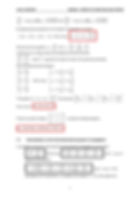
After handling Maxwell’s equations, we obtain the differential equation of propagation of the electric field E in the referential R0 (one-dimensional equation of propagation along the axis x’x):

​

The equation (1) then becomes in the referential R1 :

 

This equation would be the equation of propagation generalized to any referential assimilated to PFR.

We will see also that the crossed term  is very important. It allows us to keep the propagation of a wave (one among the two waves which are the solutions of the equation) even in a referential moving at the same speed than the first EM (Electromagnetic) wave.

​

​

7.3 Demonstration of the invariance of the generalised equation of propagation

 

Let’s now establish the extremely important result that the generalized equation of propagation keeps the same form no matter of the chosen referential assimilated to PFR or says otherwise that the generalized equation of propagation is INVARIANT by the classical law of composition of speeds (Galilean transformation).

For this, let’s show that starting from the equation (2) written in the referential R1 and going towards another ordinary referential R2 in translation at the speed V2 with regard to R0, we find back an equation of propagation of the same shape.

​

This equation is exactly the same as the one we would have obtained by going directly from the referential R0 to the referential R2.

 

This result is very important. In fact, it shows that the generalized equation (2) is consistent because it stays invariant by change of referential assimilated to PFR by using the classical transformations of coordinates (in other words, the equations (2) and (3) are identical except for the index 1 or 2).

 

Moreover, the generalized equation of propagation gives back the “classical” Maxwell’s equation by taking V1 = 0. Indeed, we then obtain: .

 

A possible solution of the generalized equation of propagation can be written :

 in the complex form or  in the real form.

 

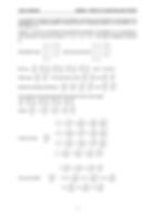
By replacing this expression in the generalized equation of propagation, we obtain:

 

 

For V1 ≠ c and V1 ≠ -c, the two solutions of this equation are:

 

Thus, very clearly, we show that the two solutions of the equation of propagation obtained from Maxwell’s equations are two waves with one propagating towards the negative x at the speed c1- = -c-V1 and the other one propagating towards the positive x at the speed c1+ = c-V1 in the referential R1.

 

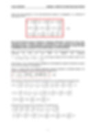
In the case where V12 = c2 (that is to say V1 = c or V1 = -c), the equation of propagation is written  and the solution  gives the following equation :

 

In the case where V1 = c and w1 ≠ 0 we have: .

An observer linked to R1 will see only one wave moving away from him at the speed c1- = -2c.

In the case where V1 = -c and w1 ≠ 0 we have: .

An observer linked to R1 will see only one wave moving away from him at the speed c1+ = 2c.

 

In the referential R0 we have:  and   and so c0- = -c and c0+ = c.

Some authors are interpreting, in my opinion wrongly, the two solutions of Maxwell’s equation of propagation as being two waves with one propagating in the future (which is normal) and the second in the past! In fact, I think that we need to interpret the two obtained waves as one going at the speed c- in the direction of the negative x and the other one going at the speed c+ in the direction of the positive x. The two obtained speeds in a referential R1 (R1 moving at the speed V1 with regard to the referential of reference R0) show well the physical signification of the two solutions of the equation of propagation of the EM waves.

 

To deepen this just a bit, we need to say that Maxwell’s equation of propagation is a differential equation of second order and so the solutions of this equation will be waves propagating with the speed vectors which will have the following properties :

• In the case of one dimension (which is the case of the calculations led until now), the extremities of the speed vectors will be equidistant from the origin in Maxwell’s Referential R0 (c0- = -c et c0+ = c) and non-equidistant from the origin in the “referential assimilated to PFR” R1 (c1- = -c-V1 and c1+ = c-V1) ;

• In the case of two dimensions, the extremities of the speed vectors will be equidistant from the origin in Maxwell’s Referential R0 (so on a circle of equation ) and on a circle of equation in the “referential assimilated to PFR” R1 in translation at the speed with regard to R0. In fact, from the equation , we deduce which is the classical composition of speeds and valid between referentials assimilated to PFR ;

• In the case of three dimensions, the extremities of the speed vectors will be equidistant from the origin in Maxwell’s Referential R0 (so on a sphere of equation ) and on a sphere of equation in the “referential assimilated to PFR” R1 in translation at the speed with regard to R0. Like in the case with two dimensions, the relation involves .

 

Demonstration in the general case with three dimensions, that the extremities of the speed vectors are on a sphere of equation  in the “referential assimilated to PFR” R1.

 

We have the relations of passage between Maxwell’s Referential R0 and a referential R1 assimilated to PFR :   which also involves:  .

The equation of propagation in Maxwell’s Referential R0 is the following :   and has for solution :

 in the complex form or  in the real form.

By starting from the real solution and by deriving, we obtain:

 

By replacing these expressions in the equation of propagation, we obtain:

 

We also have the equalities    and  .

Furthermore, for a radial luminous ray emitted by the source, we have:

    where   represents the radial unit vector of the spherical coordinates.

We can therefore write the relations:

     that is to say    .

The equation  then becomes  that is to say :  .

 

Finally, by using the relations  , we obtain the desired equation :

​

​

7.4 Generalisation of the three-dimensional equation of propagation

 

It is possible to show that in three dimensions the equation of propagation can be written:

• that is to say with i Î {x,y,z} in Maxwell’s Referential R0

 

• with i Î {x,y,z}   in the assimilated to PFR referential R1 in translation at the speed  with regard to R0.

 

It is important to note that, no matter the translation movement of the referential R1 with regard to the referential R0, it is always possible to choose the axis of x (abscissa) parallel to the movement of R1 with regard to R0.

 

However, I will give the generalized three-dimensional equation of propagation for an assimilated to PFR referential R moving at the speed   with regard to Maxwell’s referential R0.

We therefore have:      which we can also write  .

 

We have:       with E Î {Ex,Ey,Ez}

Which gives   .   In the same way, we have    and  .

Whence the following expressions :  ,    and  .

 

The expression of the partial derivative with regard to time is much longer :

 

​

Hence the final expression of the three-dimensional equation of propagation in a referential R assimilated to PFR :

 

We call the Preferred Frame of Reference “Maxwell’s Referential”, because it’s only in this referential that the “standard” equation of propagation is valid among all the referentials assimilated to PFR, or “Light Referential” because it’s the unique referential in which the light is propagating really, physically at the constant speed c in all the directions.

 

Note 1: if we want to find back an equation of propagation of the electromagnetic field identical in the referential R0 and R1, we need to “absorb” the coefficient  by the space variable, the time variable or split it on the two by taking g-1 and g (this last choice is obligatory to keep Maxwell’s equations themselves invariant and not only the equation of propagation).

 

Note 2: in certain works, (for example “Relativistic quantum mechanics” by Michael Klasen), the equation of propagation is given in the following “compact” form:

 

We are going to verify that we find back the expression (E1) by developing the expression (E2) :

 

​

We find back the equation (E1) by rewriting it in the following way:

​

​

7.5 Illustration of the equation of propagation by the calculation and the drawing of the wavefronts

 

We will illustrate all these equations by graphs obtained in a relatively easy way.

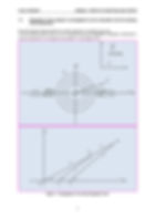
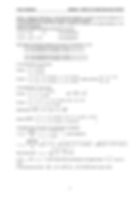
The two schemes below show a cut of a spherical EM wave propagating in Maxwell’s referential R0 and the referential R1 (in translation at the speed  with regard to R0).

​

Written in Maxwell’s Referential or Light Referential, Maxwell’s equations involve the existence of a EM wave propagating at the speed of modulus c no matter the direction.

In the referential R1 it’s much more complex, because the modulus of the speed depends on the direction of propagation.

If we use the polar coordinates (3D spherical), we have:

​

We consider the EM wave emitted by the source in the direction q0 in R0 :

• at t in the referential R0 the wave is in M0(x0, y0) º (r0, q0)

• at t in the referential R1 the wave is in M1(x1, y1) º (r1, q1)

 

• at t’ in the referential R0 the wave is in M’0(x’0, y’0) º (r’0, q’0)

• at t’ in the referential R1 the wave is in M’1(x’1, y’1) º (r’1, q’1)

 

The speed vector of the light in the referential R1 is therefore :

   and its modulus is :

We can also write :    

or   which shows that the extremities of the speed vectors    are on a circle.

In the same way, we have :    which is also a circle.

 

Note 1 : this formula is general to any spherical wave by setting oneself in the plan   with .

 

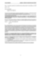
The curves of the following pages show well the “deformation” of the waves in a referential assimilated to PFR in translation with regard to Maxwell’s Referential or the Light Referential.

These curves are the same as those seen by the pilot of a plane flying over a pond on whose surface concentric wavelets would propagate.

The remarkable point here is that these curves correspond to waves obtained from the equation of propagation deduced by a classical transformation of a referential assimilated to PFR to another one.

 

As for me, these curves reassure me because the Special Relativity forbids that the speed of translation of a referential with regard to another one would be higher than the speed of light (it’s the famous  which imposes this).

 

By a “thought-experiment”, that is to say an experiment described by the thought but not achievable (Einstein himself liked using “thought-experiments”), we can imagine very well a referential moving two times, ten times or one thousand times faster than the speed of light. How would the EM waves look like in such referential? Einstein’s Relativity doesn’t even allow us to ask ourselves the question.

I hope that the present chapter will start to convince the reader that the introduction of a Preferred Frame of Reference (Maxwell’s Referential or Light Referential) in which the EM waves are propagating at the same speed c in all the directions as well as the introduction of Maxwell’s equations generalized to any referential assimilated to PFR in translation with regard to the Light Referential is legitimate.

 

We will see in an upcoming chapter that the use of this Light Referential in the frame of the gravitation is very fruitful because it allows us to establish an equivalence between the Light Referential which is modified by the gravitation and Einstein’s General Relativity.

 

A big part of the theory presented in this work is based on the fact that the equations such as Maxwell wrote them are physically exact solely in a Preferred Frame of Reference that I call Maxwell’s Referential or Light Referential.

The definition of Maxwell’s Referential is that the equations written by Maxwell are physically true only in this referential.

The definition of the Light Referential is that the light is propagating really, physically at the constant speed c in all the directions only in this referential.

 

These two referentials with two different definitions are actually one and only referential.

​

It is very important to indicate that the effects of Einstein’s Special Relativity apply to the MATTER in the broad sense and to the INSTRUMENTS OF MEASURE (constituted of course of matter), which means that:

• a clock linked to a matter referential R1 moving at the speed with regard to R0 will beat physically slower but this clock can be considered as “disturbed” or “distorted” (even if we know how to calculate exactly the error) with regard to the time of reference of the Preferred Frame of Reference;

• a ruler linked to a matter referential R1 moving at the speed with regard to R0 will have a length physically shorter than in R0, but this ruler can be considered as “disturbed” or “distorted” (even if we know how to calculate exactly the error) with regard to the Preferred Frame of Reference (which is identical to the Referential of Maxwell-Light);

• the speed of the light then constant with instruments constituted of matter (clocks and rulers “distorted” by the speed they have with regard to the Preferred Frame of Reference) but the existence of a makes that the light undergoes the classic composition of speeds by using the referentials assimilated to PFR.

 

We will see in an upcoming chapter that it’s the same for GRAVITATION which effects apply on the MATTER in the broad sense and on the MEASURING INSTRUMENTS (rulers, clocks).

​

​

7.6 Conclusion

 

This chapter about the generalized equation of propagation of the light deduced from Maxwell’s equations and obtained in a referential assimilated to PFR in uniform rectilinear translation of speed V with regard to the Preferred Frame of Reference and retaining by the thought clocks of same period and rulers of same length that the ones of the Preferred Frame of Reference is very interesting for several reasons :

• the generalized equation of propagation gives back the well-known equation when V = 0;

• the generalized equation of propagation is , that is to say that if we consider the generalized equation of propagation for an electromagnetic wave written in the referential R1 in movement at the speed VR1/PFR with regard to the Preferred Frame of Reference, and that we apply the classical transformations of coordinates (classical composition of speeds with VR2/R1 = VR2/PFR – VR1/PFR), we fall back on the generalized equation of propagation for this same electromagnetic wave written in the referential R2 in movement at the speed VR2/PFR with regard to the Preferred Frame of Reference ;

• the wave surfaces found (spheres in three-dimension) with the generalized equation of propagation correspond correctly to the vision that would have an observer in uniform rectilinear translation with regard to the Preferred Frame of Reference and endowed with the same clocks and rulers than the ones of the Preferred Frame of Reference.

 

In his book « Mécanique quantique relativiste » Michael Klasen writes :

« The equations of the movement of the classical mechanics of the fields are not covariant under the Galilean transformations : the equation of the movement of a field y(x’,t’) propagating at the speed c in the referential S’,  , where  , becomes    in the referential S. Thus it is not covariant. »

​

In the frame of my theory, we should rather write :

« The equation   is the generalized equation of propagation. It is invariant by the Galilean transformation. And the equation   is the form of the generalized equation in the unique case where it is expressed in the Preferred Frame of Reference defined by the medium of propagation of the electromagnetic waves. »

 

 

To be more comprehensive, we have to add that for modern science :

Whatever the Galilean referential in which the experiments are realized, they lead to the fact that we have to use the « standard » equation of propagation . From there, it is possible to deduce that the light propagates in all the inertial referentials and in all the directions with the universal speed c (principle of constancy of the speed of light of Einstein’s special relativity).

 

In the frame of my theory, it is proposed that :

Einstein’s Special Relativity is a theory of observation and measurement. The used instruments (material rulers and clocks) are distorted because of their speed with regard to the Preferred Frame of Reference which leads to measure a constant speed of light.

In a referential assimilated to PFR in which the rulers have the same length and the clocks the same period that the ones situated in the Preferred Frame of Reference, the light undergoes the classical composition of speeds (thus the speed of light is not constant) and we have to used the generalized equation of propagation.

 

The essential point of this chapter is that the generalized equation of propagation exists, that it is invariant by the Galilean transformation and that it possesses a real and physical signification in all the referentials assimilated to PFR.